Bond and stock valuation concepts
Every financial asset, at its core, is simply a contractual claim on future cash flows. Whether a client is holding a thirty-year municipal bond to fund their retirement or shares of a multinational technology conglomerate for long-term growth, the fundamental question of valuation remains identical: what is the precise worth today of money that will not arrive until tomorrow? For the financial planner, the ability to answer this question separates pure speculation from disciplined investment management. You are not just picking securities; you are systematically pricing the future. To do this accurately, we must understand how to construct the bridge between future expected cash and present intrinsic value, adjusting for time, risk, and growth.
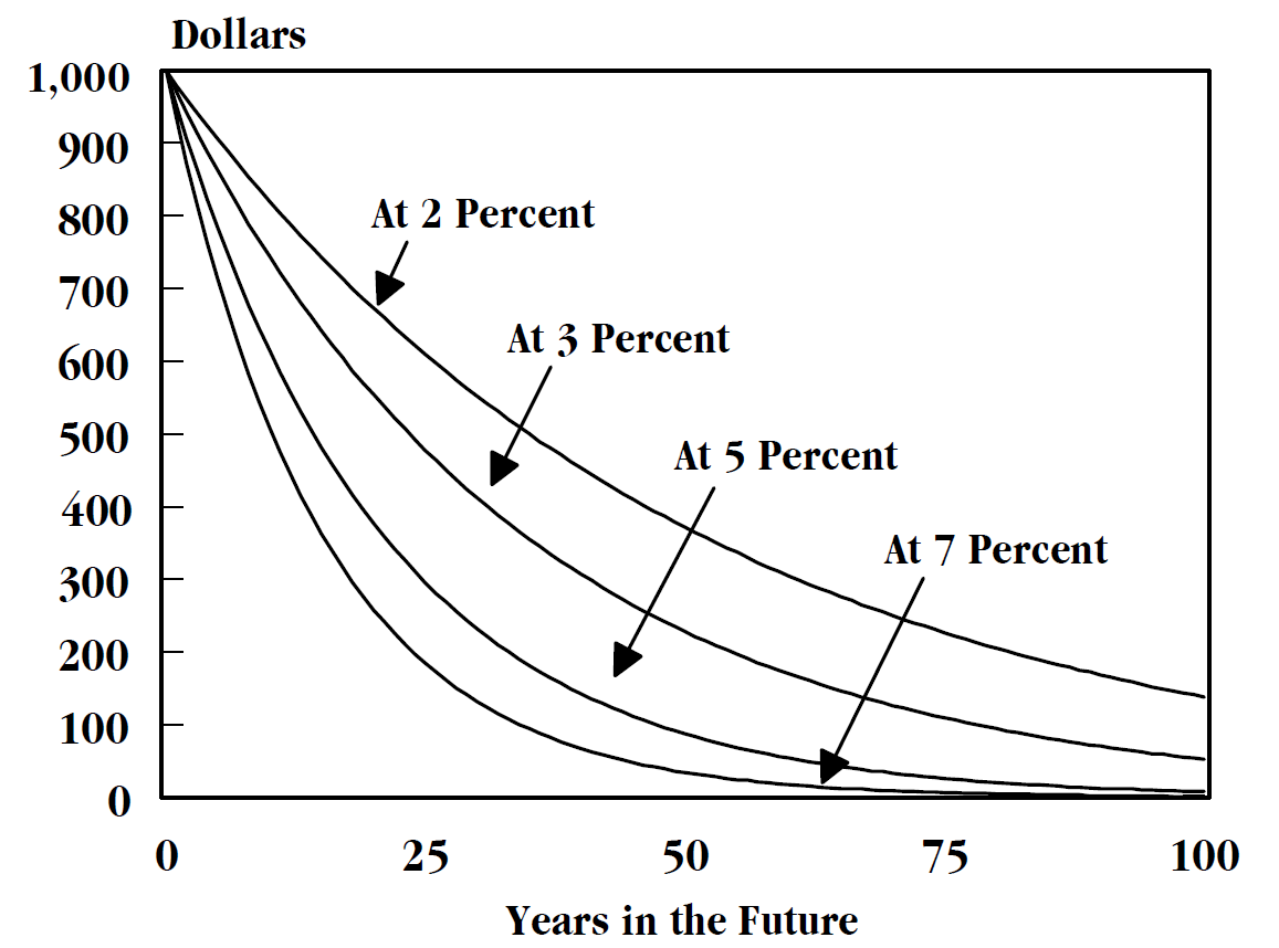
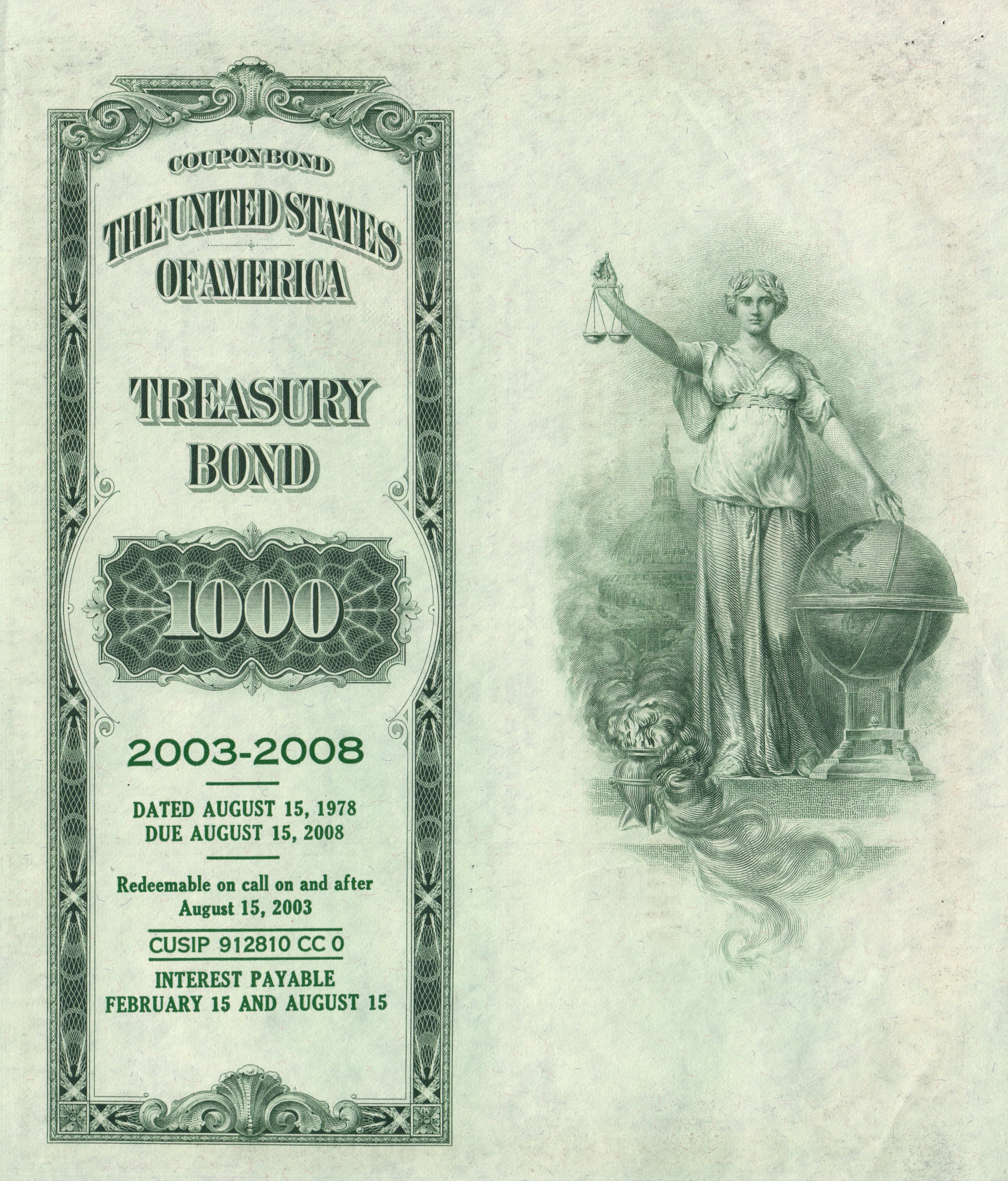
When your client buys a bond, they are lending capital in exchange for a highly specific set of promises. The intrinsic value of a bond equals the present value of all expected future cash flows discounted at the required yield to maturity.
To build this present value, we must first identify what those cash flows are. A bond's future cash flows consist of periodic coupon payments and the return of the principal par value at maturity. Imagine a stream of small, steady payments (the coupons) followed by one massive reservoir of water released at the very end (the par value).
But how do we measure the return on this instrument? Planners must distinguish between three distinct yield metrics:
- The Coupon Rate: The static, stated percentage of par value paid annually.
- Current Yield: A snapshot metric. The current yield of a bond equals the annual coupon payment divided by the current market price of the bond. It tells your client what the bond is paying relative to what it costs today, but it completely ignores the capital gain or loss realized at maturity.
- Yield to Maturity (YTM): The ultimate measure of a bond's economic reality. Yield to maturity represents the total annualized return an investor earns if a bond is held to maturity and all coupons are reinvested at the same yield.
Crucial Exam Trap: The reinvestment assumption is the Achilles' heel of the YTM calculation. If market rates fall, your client cannot reinvest their coupons at the original YTM, introducing reinvestment rate risk.
The Price-Yield Seesaw
The financial universe is governed by an inescapable physical law: Bond prices and market interest rates have an inverse relationship. When new bonds are issued at higher rates, existing bonds with lower coupons become less attractive, forcing their prices down.
This inverse relationship creates three possible pricing scenarios for any bond:
| Pricing State | Condition | Intuition for the Client |
|---|---|---|
| Discount | A bond sells at a discount when the required yield to maturity is greater than the stated coupon rate. | The bond's coupon is "too low" for the current market. To compensate the buyer, the price must drop below par. |
| Par | A bond sells exactly at par value when the required yield to maturity equals the stated coupon rate. | The bond's coupon matches exactly what the market demands. No price adjustment is needed. |
| Premium | A bond sells at a premium when the required yield to maturity is less than the stated coupon rate. | The bond is paying a generously high coupon compared to current market rates. Buyers will pay extra (above par) for this privilege. |
Knowing that bond prices move inversely to interest rates is only the first step. The professional planner must answer the client's next, more urgent question: "If rates go up 1%, exactly how much money will I lose?"
To answer this, we measure the bond's center of gravity.
Macaulay Duration: The Balancing Point of Time
Imagine a physical seesaw with a timeline mapped along the board. The coupon payments are small weights placed along the board, and the principal repayment is a massive boulder sitting at the very end (the maturity date). Where must you place the fulcrum so the board balances perfectly? That fulcrum is Macaulay duration.
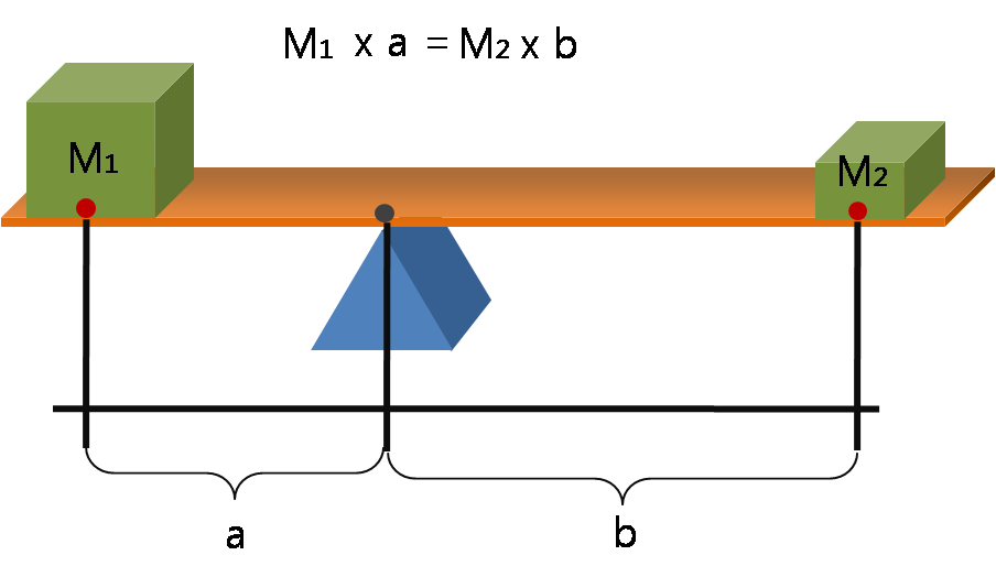
Macaulay duration measures the weighted average time until the cash flows of a bond are received. Because it measures time, Macaulay duration is expressed in units of years.
The mechanics of this balancing point give us strict rules:
- The Macaulay duration of a zero-coupon bond is exactly equal to the time remaining until the bond's maturity. (There are no intermediate coupons, so the entire weight sits at the very end).
- The Macaulay duration of a coupon-paying bond is always less than the time remaining until the bond's maturity. (The intermediate coupon payments pull the fulcrum/balancing point forward).
Three variables act as levers on a bond's duration. Grasping these is essential for portfolio construction:
- Maturity: Longer-maturity bonds generally have higher durations than shorter-maturity bonds. A bond paying out in 30 years has a center of gravity much further out than a 2-year note.
- Coupon: Lower-coupon bonds generally have higher durations than higher-coupon bonds. If a bond pays tiny coupons, more of its total value is heavily weighted toward that final par payment at maturity, pushing the fulcrum outward.
- Yield: Lower-yielding bonds generally exhibit higher durations than higher-yielding bonds. When yields are low, future cash flows aren't discounted as heavily, keeping more of their "weight" intact out in the future.
Modified Duration: Translating Time into Price Sensitivity
While Macaulay duration gives us a measure of time, time alone doesn't tell us how much a bond's price will fluctuate. We must mathematically adjust it.
Modified duration equals the Macaulay duration divided by one plus the yield to maturity per payment period.
What does this new number tell us? Modified duration measures the approximate percentage change in a bond's price for a one percent change in interest rates. Consequently, a higher duration indicates a higher sensitivity of a bond's price to interest rate fluctuations. If a client holds a bond fund with a modified duration of 8.0, and interest rates rise by 1%, you can confidently estimate the fund's net asset value will drop by approximately 8%.
The Flaw of Duration: Convexity
Duration is an incredibly powerful tool, but it is fundamentally flawed. Duration formulas assume a linear relationship between bond prices and interest rate changes. They draw a straight, tangent line against a curve.
In reality, a bond's price does not drop in a perfectly straight line as yields rise. The actual price curve bows outward like a smile. Bond convexity measures the curvature in the relationship between bond prices and bond yields.
Why does this matter to the practitioner? Because convexity accounts for the non-linear relationship between bond prices and interest rate changes. Convexity shows us that as yields fall, bond prices actually rise faster than duration predicts. And as yields rise, bond prices fall slower than duration predicts. Convexity is highly desirable; it is the mathematical cushion that protects your client's fixed-income portfolio when rates surge.
While a bond promises legally binding cash flows, a share of stock promises nothing. Yet, the foundational law of valuation remains unchanged. The intrinsic value of a stock represents the present value of all expected future dividends.
The challenge lies in the word "expected." How do we value a stream of cash flows that might grow, shrink, or continue forever?
The Dividend Discount Model (DDM)
To bring order to this chaos, we use models to forecast that infinite stream. The most famous of these is the Gordon Growth Model, which is a dividend discount model assuming dividends grow at a constant rate indefinitely.
The elegance of the Gordon Growth Model lies in its simplicity. It collapses an infinite series of future dividends into a single, clean equation. The Gordon Growth Model calculates stock value by dividing the expected dividend in year one by the difference between the required rate of return and the dividend growth rate.
The Gordon Growth Model Formula: V0=r−gD1 Where V0 is the intrinsic value, D1 is the expected dividend next year, r is the required rate of return, and g is the constant growth rate.
To use this model successfully on the exam, you must respect its exact inputs:
- Finding D1: You cannot use today's dividend. The expected dividend in year one equals the current dividend multiplied by one plus the expected dividend growth rate (D1=D0×(1+g)).
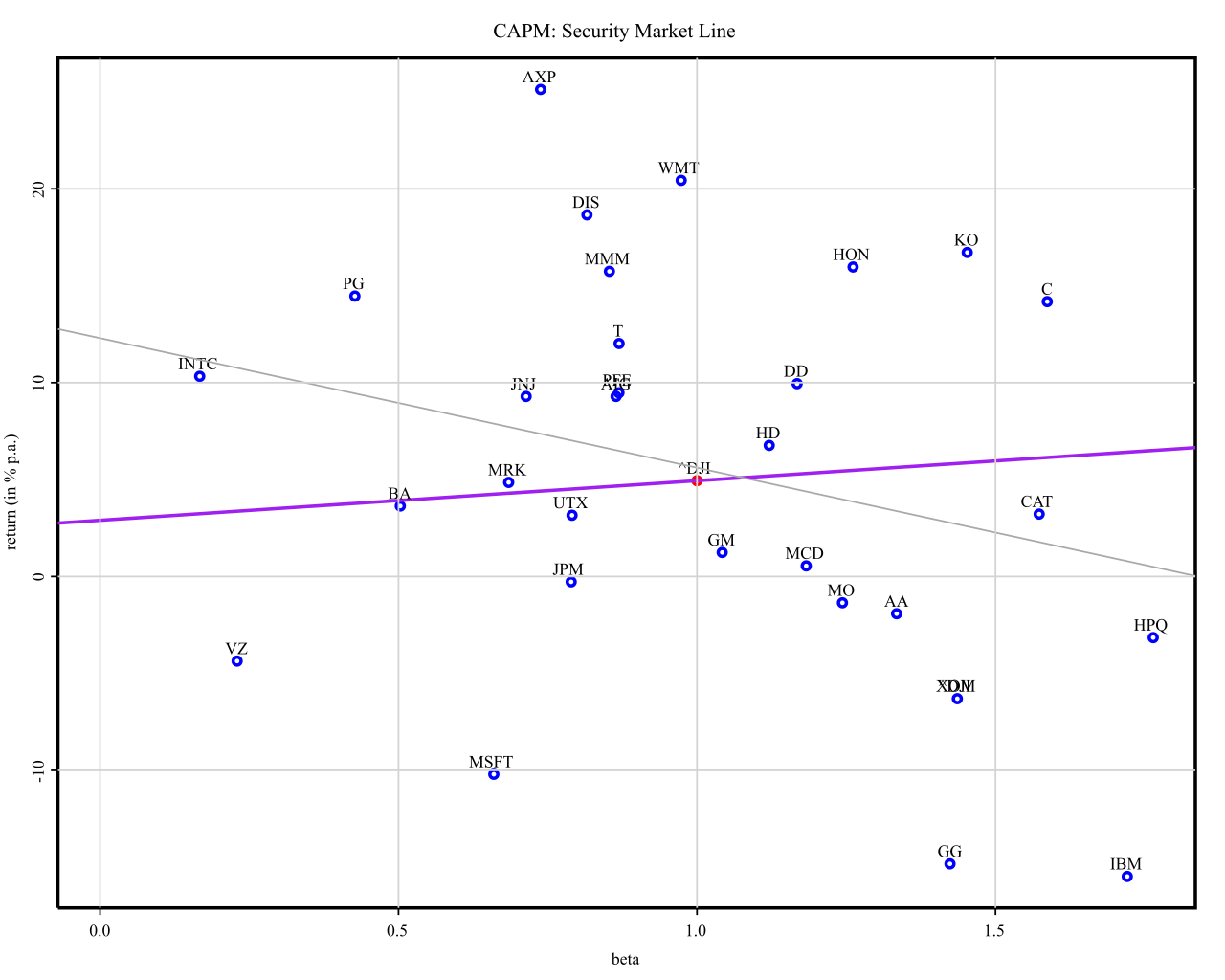
- The Required Rate (r): What return does the client demand for taking on this equity risk? The required rate of return used in dividend discount models is frequently calculated using the Capital Asset Pricing Model (CAPM).
- The Mathematical Constraint: The Gordon Growth Model requires the investor's required rate of return to be strictly greater than the assumed dividend growth rate. If g were greater than r, the denominator would be negative, yielding a mathematically impossible negative stock price.
This model allows us to observe how sensitive a stock's price is to our economic assumptions.
- If the Federal Reserve raises rates, or if the stock becomes riskier, the required rate of return (r) goes up. Mathematically, a larger denominator shrinks the outcome. Therefore, an increase in the required rate of return decreases the intrinsic value of a stock calculated using the dividend discount model.
- Conversely, if the company invents a brilliant new product, their growth trajectory changes. A larger g shrinks the denominator. Thus, an increase in the expected dividend growth rate increases the intrinsic value of a stock calculated using the dividend discount model.
The Gordon Growth Model is beautiful in theory, but practically, many companies (like early-stage tech firms) do not pay dividends. How do we value them? We shift from absolute valuation to relative valuation, primarily through earnings multiples.
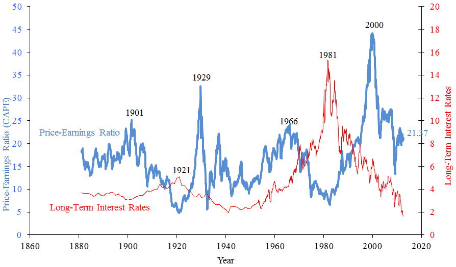
The Price-to-Earnings (P/E) ratio measures a company's current share price relative to the company's earnings per share. It essentially tells you how much investors are willing to pay for $1 of a company's earnings.
When reviewing a stock research report, you will encounter two distinct flavors of this metric:
- Trailing P/E: Looking at the firm's historical track record. Trailing Price-to-Earnings ratios are calculated using the earnings per share from the most recent twelve months.
- Forward P/E: Looking through the windshield instead of the rearview mirror. Forward Price-to-Earnings ratios are calculated using forecasted earnings per share for the upcoming twelve months.
We can use these multiples to construct a target price for a stock. To estimate intrinsic value using the Price-to-Earnings approach, an analyst multiplies the expected earnings per share by a benchmark Price-to-Earnings multiple. (For example, if you project a company will earn $4.00 per share next year, and its peer group historically trades at a 15x P/E multiple, the estimated intrinsic value is $60.00).
Growth, Value, and the PEG Ratio
Because investors are paying for future potential, P/E ratios are intimately tied to growth expectations. Growth stocks typically trade at higher Price-to-Earnings ratios compared to value stocks. The market willingly pays a premium—perhaps a 40x P/E—for a software company expected to double its earnings every three years.
Conversely, value investors typically seek stocks with Price-to-Earnings ratios that are lower than the broader market average. They are looking for companies that have been unfairly beaten down by the market, trading at an unwarranted discount.
But how do we compare a high-P/E growth stock to a low-P/E value stock on an apples-to-apples basis? We introduce growth into the equation.
The Price/Earnings-to-Growth (PEG) ratio is calculated by dividing a stock's Price-to-Earnings ratio by the company's expected annualized earnings growth rate.
If a stock has a P/E of 20 and an expected growth rate of 20%, its PEG ratio is 1.0. If a seemingly "cheap" value stock has a P/E of 10 but is only growing at 2%, its PEG ratio is a staggering 5.0. By looking at the PEG ratio, the financial planner realizes that a high P/E ratio might actually represent a bargain if the company's growth rate is high enough to justify the price.
Whether calculating the modified duration of a municipal bond to protect a retiree's income, or assessing the forward P/E of an equity to build a wealth-accumulation portfolio, these valuation principles are the diagnostic tools of your profession. They transform market noise into quantifiable, structured reality.