Quantitative investment concepts and measures of investment returns

Judging an investment solely by its annualized return is like evaluating a ship's voyage purely by whether it reached port, ignoring the fact that the passengers spent the entire journey violently seasick. In financial planning, the turbulence of the journey dictates whether a client remains invested long enough to realize their expected returns. When a client abandons a meticulously crafted financial plan during a market correction, it is rarely because the long-term math was wrong; it is because the experiential reality of the risk exceeded their tolerance. Therefore, to construct durable portfolios and evaluate the true skill of the managers running them, we must rigorously quantify risk and isolate exactly where a portfolio's returns are coming from. We accomplish this by dissecting total risk, mapping how assets move together, and measuring performance against a standardized baseline of market exposure.

When we look at an investment's historical track record, the average return only tells us the center of gravity. We need to know the spread of the data around that center. Standard deviation measures the total risk of an investment. It represents the dispersion of investment returns around the historical average return.

Standard deviation is rooted in the mathematical concept of variance. Specifically, standard deviation is calculated as the square root of variance.

Standard Deviation ( $\sigma$ ) $= \sqrt{\text{Variance}}$

Two probability distributions with the same historical average but different standard deviations. The blue distribution has higher total risk due to its wider dispersion of potential outcomes.

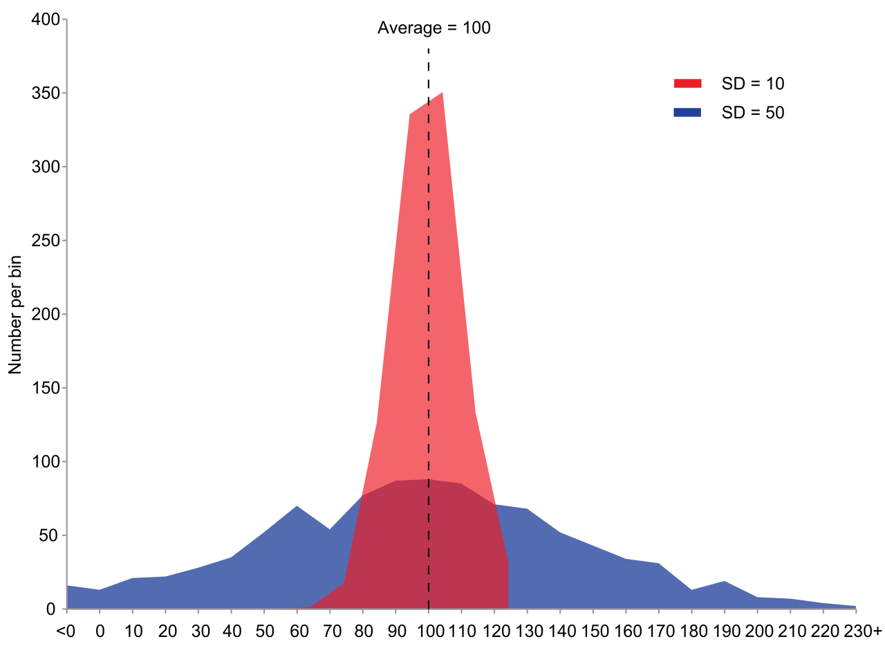
A higher standard deviation indicates greater volatility and higher total risk for an investment. When advising a client, standard deviation provides a probabilistic map of what they can expect to experience in any given year. Assuming investment returns roughly follow a normal distribution (a bell curve), we can apply the empirical rule to set precise client expectations:

In a normal distribution, approximately 68 percent of returns fall within one standard deviation of the mean.
In a normal distribution, approximately 95 percent of returns fall within two standard deviations of the mean.
In a normal distribution, approximately 99 percent of returns fall within three standard deviations of the mean.

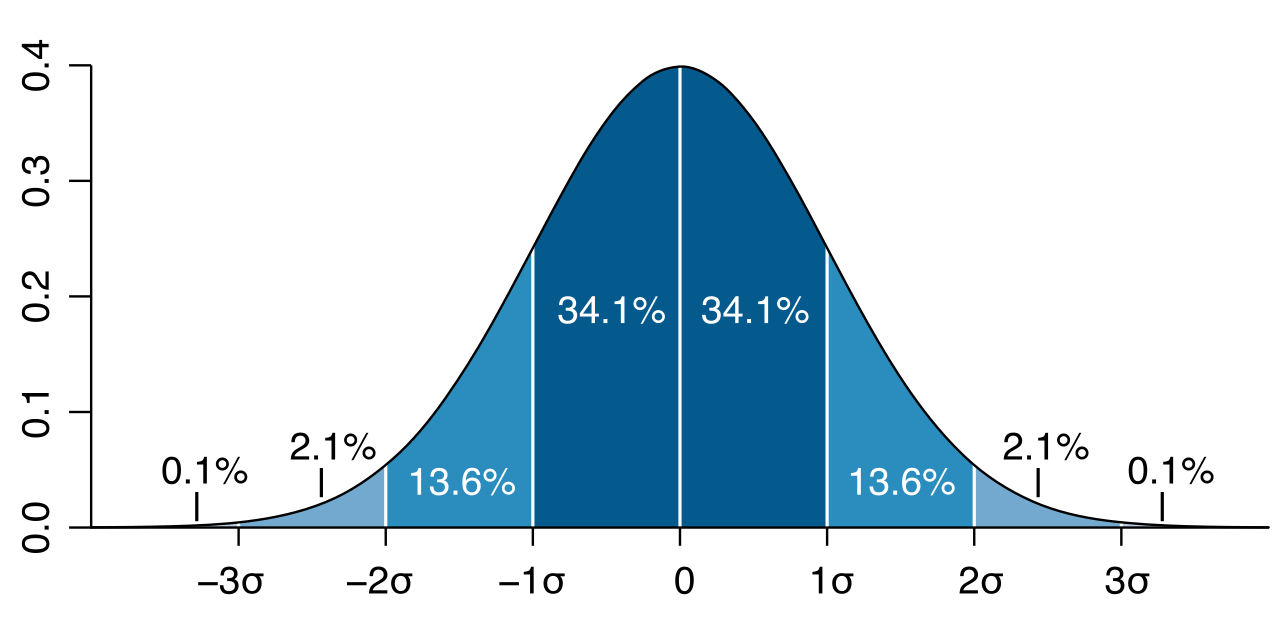
A normal distribution curve demonstrating the empirical rule, where roughly 68%, 95%, and 99.7% of returns fall within one, two, and three standard deviations of the mean, respectively.

If a mutual fund has an expected average return of $8\%$ and a standard deviation of $10\%$ , you can confidently explain to your client that there is a 95 percent probability their actual return in any single year will land somewhere between $-12\%$ and $+28\%$ (the average minus and plus two standard deviations).

Portfolios are not built in isolation; they are complex systems of interacting assets. To understand how combining assets affects total portfolio risk, we must measure how those assets interact with one another.

Covariance

Covariance measures the directional relationship between the returns of two distinct assets.

A positive covariance indicates that two assets tend to move in the same direction.
A negative covariance indicates that two assets tend to move in opposite directions.

While covariance tells us the direction of the relationship, its mathematical output is not standardized, making it difficult to interpret the strength of that relationship.

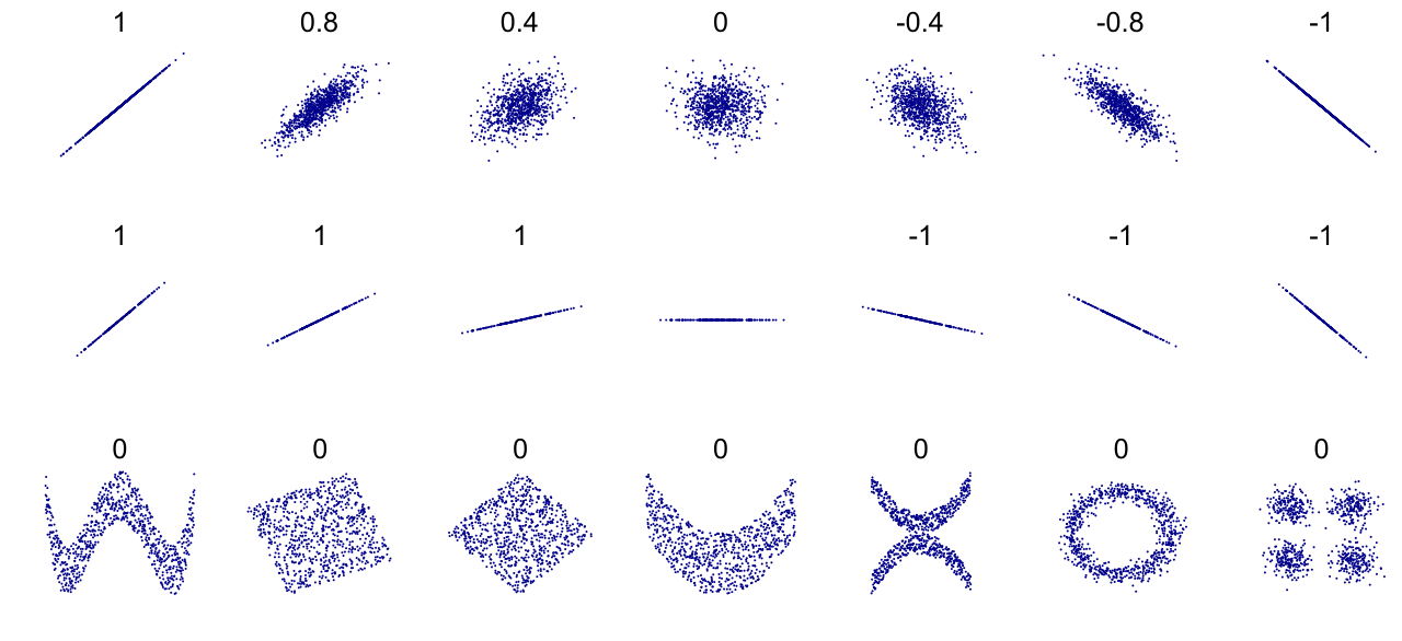
The Correlation Coefficient

To standardize covariance, we use the correlation coefficient, which measures the degree to which the returns of two assets move in relation to each other. The correlation coefficient is represented by the variable R and ranges strictly from negative 1.0 to positive 1.0.

A correlation coefficient of positive 1.0 indicates perfect positive correlation between two assets. They move in lockstep.
A correlation coefficient of negative 1.0 indicates perfect negative correlation between two assets. They move in exact opposite directions.
A correlation coefficient of zero indicates no linear relationship between the returns of two assets.

Scatterplots demonstrating various correlation coefficients. A correlation of 1.0 or -1.0 indicates a perfect linear relationship, while a correlation of 0 indicates the absence of a linear relationship.

Mathematical Relationship Covariance can be calculated by multiplying the correlation coefficient by the standard deviation of each asset: $\text{Covariance} = R \times \sigma_{\text{Asset 1}} \times \sigma_{\text{Asset 2}}$

The correlation coefficient is the engine of modern portfolio diversification. Combining assets with a correlation coefficient of less than positive 1.0 provides diversification benefits by reducing the portfolio's overall standard deviation. In the extreme theoretical case, combining two assets with a perfect negative correlation (-1.0) allows an investor to construct a zero-risk portfolio, as the volatility of one asset perfectly cancels out the volatility of the other.

Standard deviation measures total risk—the sum of both the risk inherent to the specific company (unsystematic risk) and the risk of the broader economic system. However, in a highly diversified portfolio, the company-specific risks cancel each other out. What remains is systematic risk, which is also known as market risk or non-diversifiable risk.

We measure systematic risk using Beta. Beta measures the systematic risk of an investment relative to a benchmark index. By definition, the benchmark market index always has a beta of exactly 1.0.

A beta greater than 1.0 indicates that an investment is more volatile than the overall market. (e.g., a beta of 1.2 implies the asset will move 20% more than the market).
A beta less than 1.0 indicates that an investment is less volatile than the overall market.

Beta mathematically bridges the specific asset and the broader market. The formula for beta is the covariance of the asset and the market divided by the variance of the market. Alternatively, using our knowledge of standard deviation and correlation, beta can be calculated by multiplying the correlation coefficient by the quotient of the asset standard deviation over the market standard deviation.

Beta Calculation $\beta = \frac{\text{Covariance}_{\text{Asset, Market}}}{\text{Variance}_{\text{Market}}}$

$\beta = R \times \left( \frac{\sigma_{\text{Asset}}}{\sigma_{\text{Market}}} \right)$

If standard deviation is total risk and beta is only market risk, how do you know which metric to use when evaluating a mutual fund? You must ask a fundamental question: How much of this fund's total volatility is actually caused by the broader market?

We answer this using the coefficient of determination, which is represented by R-squared ( $R^2$ ).

The coefficient of determination measures the percentage of a portfolio's return variations explained by the benchmark market index movements. Mathematically, the coefficient of determination is calculated simply by squaring the correlation coefficient ( $R$ ).

If an investment has a correlation with the S&P 500 of $0.90$ , its R-squared is $0.81$ (or 81%). This tells us that 81% of the mutual fund's price movements are directly explained by what the S&P 500 is doing.

Visualizing R-squared: The linear regression model (right) demonstrates how effectively a benchmark index explains the variance in an asset's returns compared to a simple historical average (left). The closer R-squared is to 1, the tighter the fit.

This leads to a critical rule for the CFP® exam and real-world performance evaluation:

An R-squared value of 0.70 or higher indicates that beta is a reliable measure of the portfolio risk, because the portfolio is sufficiently diversified and tracks the market closely.
An R-squared value below 0.70 indicates that beta is not a reliable measure of the portfolio risk. The portfolio's movements are driven largely by internal, unsystematic factors rather than the benchmark.
Crucially: If a portfolio has an R-squared below 0.70, standard deviation must be used as the primary risk measure instead of beta.

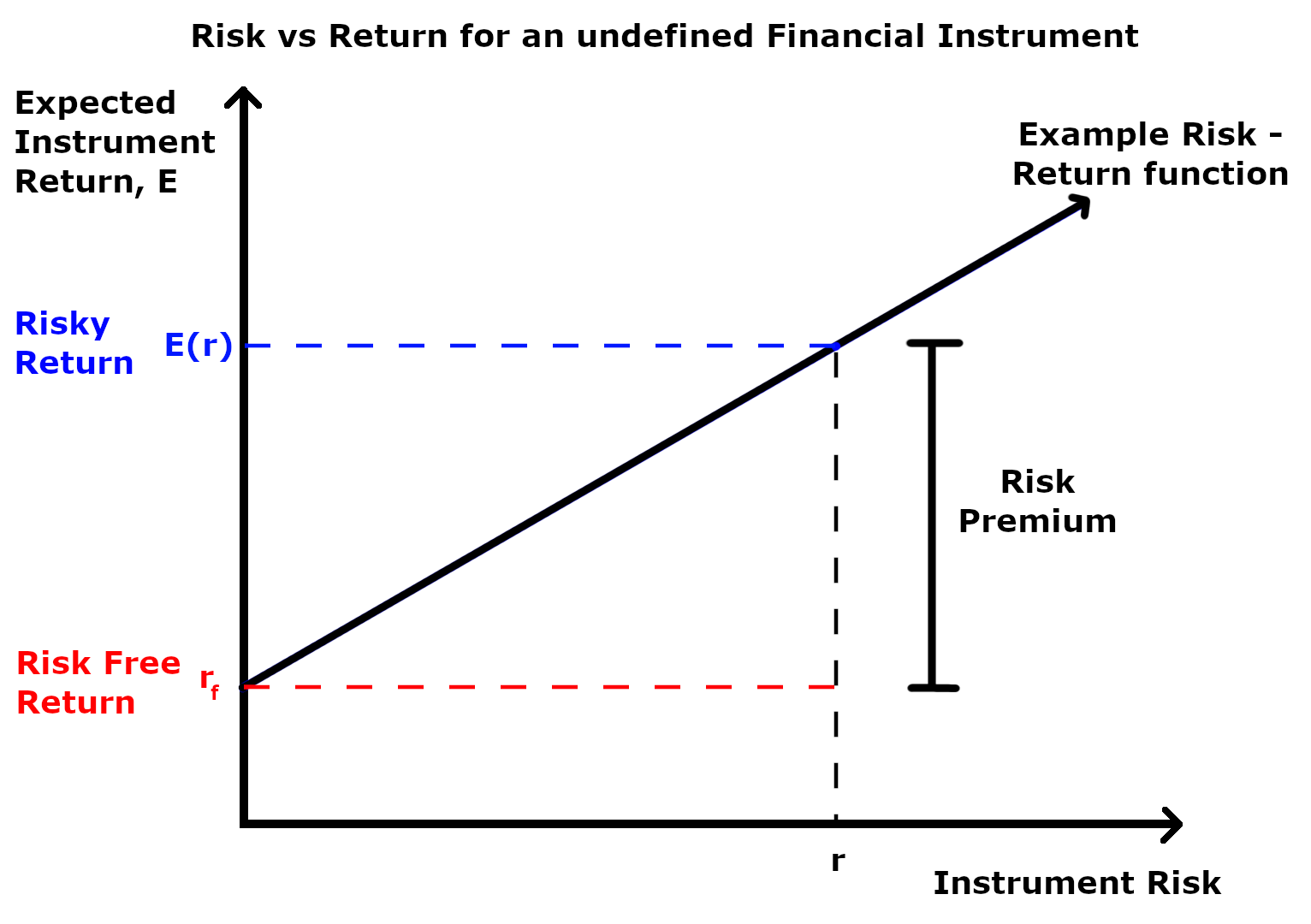
If an investor decides to take on market risk, they must be compensated for it. The baseline for all investment returns is the risk-free rate, which is typically represented by the yield on a 90-day United States Treasury bill.

A historical U.S. Treasury Bill. Short-term T-bills are universally utilized in financial models as the baseline risk-free rate due to their virtually non-existent default risk.

If an investor moves their money from a risk-free 90-day T-bill into the stock market, they expect an additional layer of return. We call this the market risk premium. The market risk premium is calculated by subtracting the risk-free rate from the expected return of the market.

Using beta, the risk-free rate, and the market risk premium, we can determine exactly how much return an asset should generate given its systematic risk. This is the Capital Asset Pricing Model (CAPM).

CAPM Expected Return $= \text{Risk-Free Rate} + [\beta \times \text{Market Risk Premium}]$

The CAPM risk-return function illustrates how the expected return of an asset increases proportionally to the level of systematic risk taken above the baseline risk-free rate.

Note: Because the Market Risk Premium is defined as (Expected Market Return - Risk-Free Rate), the CAPM expected return is calculated by adding the risk-free rate to the product of beta and the market risk premium.

When a client pays an active mutual fund manager, they are paying for outperformance. But a manager who achieves a 15% return by taking on massive, reckless risk is not necessarily skilled; they are just highly leveraged. To evaluate true skill, we must use risk-adjusted performance measures.

The Sharpe Ratio

The Sharpe ratio measures risk-adjusted return by dividing a portfolio risk premium by the portfolio standard deviation. The portfolio risk premium in the Sharpe ratio is the portfolio actual return minus the risk-free rate.

Sharpe Ratio $= \frac{\text{Actual Return} - \text{Risk-Free Rate}}{\text{Standard Deviation}}$

Because the Sharpe ratio uses standard deviation, it evaluates performance based on total risk. This means it accounts for both systematic and unsystematic risk. Therefore, the Sharpe ratio is the most appropriate performance measure for a poorly diversified portfolio (where unsystematic risk is high). A higher Sharpe ratio indicates better historical risk-adjusted performance.

The Treynor Ratio

The Treynor ratio measures risk-adjusted return by dividing a portfolio risk premium by the portfolio beta. Like the Sharpe ratio, the portfolio risk premium in the Treynor ratio is the portfolio actual return minus the risk-free rate.

Treynor Ratio $= \frac{\text{Actual Return} - \text{Risk-Free Rate}}{\text{Beta}}$

Because the Treynor ratio uses beta, it evaluates performance based strictly on systematic risk. It assumes unsystematic risk has been eliminated. Thus, the Treynor ratio is an appropriate performance measure for a well-diversified portfolio. A higher Treynor ratio indicates better historical risk-adjusted performance relative to market risk.

Sharpe vs. Treynor Quick Reference

Feature	Sharpe Ratio	Treynor Ratio
Risk Measure Used	Standard Deviation	Beta
Type of Risk Evaluated	Total Risk	Systematic Risk
Appropriate Portfolio	Poorly Diversified (or standalone)	Well-Diversified
Numerator	Actual Return - Risk-Free Rate	Actual Return - Risk-Free Rate

Jensen's Alpha

While Sharpe and Treynor provide relative ratios, Jensen's Alpha measures absolute performance. It calculates the absolute excess return of a portfolio over the expected return calculated by the Capital Asset Pricing Model.

Jensen's Alpha is calculated by subtracting the Capital Asset Pricing Model expected return from the portfolio actual return.

Jensen's Alpha $= \text{Actual Return} - \text{CAPM Expected Return}$

A positive Jensen's Alpha indicates that the portfolio manager outperformed the market on a risk-adjusted basis. They generated more return than the CAPM dictates they should have for the level of risk taken.
A negative Jensen's Alpha indicates that the portfolio manager underperformed the market on a risk-adjusted basis.

Because Jensen's Alpha requires beta as an input to calculate the expected return via the Capital Asset Pricing Model, it shares the same constraints as the Treynor ratio. Jensen's Alpha relies on the assumption that beta is a reliable measure of risk for the portfolio (meaning $R^2 \ge 0.70$ ). Consequently, Jensen's Alpha is an appropriate performance measure only for well-diversified portfolios.