Retirement income and distribution strategies
Imagine an engineer tasked with draining three interconnected reservoirs to sustain a city for thirty years, knowing the rainfall is utterly unpredictable. If they drain the wrong reservoir first, the water evaporates faster than it can replenish. If a drought hits in the first three years and they draw down at the same rate, the system permanently collapses. This is the precise mathematical reality of retirement distribution planning. Accumulating capital is a problem of addition and multiplication; distributing it is a complex problem of fluid dynamics involving taxation, compounding, and market volatility. For a financial planner, the objective is not just reaching a target number, but engineering a withdrawal architecture that maximizes portfolio longevity while surviving the unpredictable elements of the market.

To maximize longevity, we must first minimize the friction in the system. In retirement planning, that friction is taxes. How you sequence withdrawals from various account types determines how much of the portfolio is preserved to generate future returns.
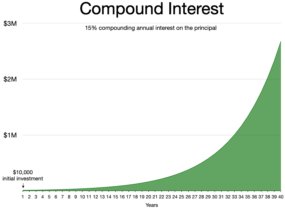
The traditional rule of thumb for retirement withdrawals dictates withdrawing from taxable accounts first. Why? Because you are allowing the mathematics of compounding to work in a protected vacuum for as long as possible. The traditional withdrawal sequence suggests accessing tax-deferred accounts (like traditional IRAs and 401(k)s) after exhausting taxable accounts. Finally, the traditional withdrawal sequence places tax-free accounts like Roth IRAs last in the distribution order. Delaying withdrawals from tax-advantaged accounts maximizes the compounding of tax-deferred or tax-free growth. By leaving the Roth IRA untouched until the end, you allow the most tax-efficient dollars to experience the longest period of uninterrupted, tax-free compounding.
Let's look at the tax mechanics governing these reservoirs:
- Taxable Accounts: Selling assets in a taxable account incurs taxes only on the realized capital gains or earned interest, not on the return of your original principal. Furthermore, long-term capital gains from taxable account distributions are typically taxed at lower federal rates than ordinary income.
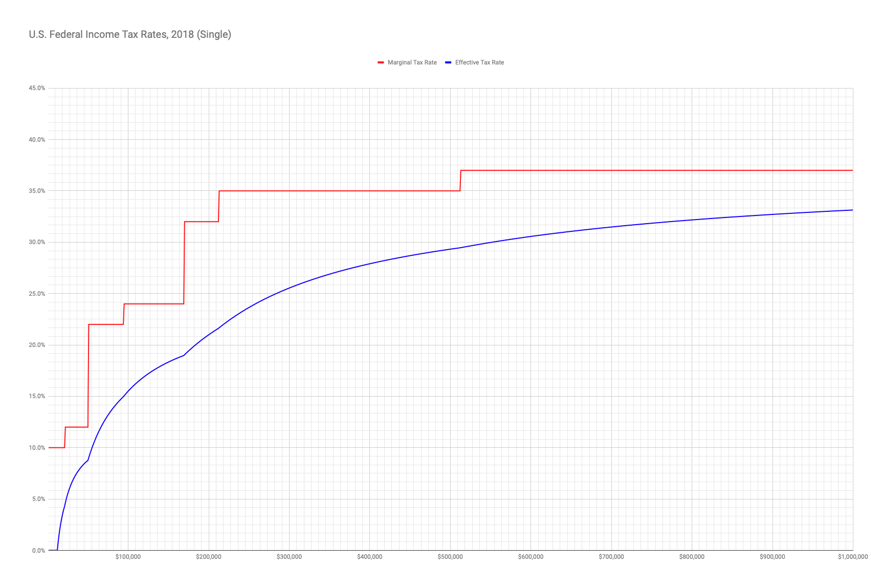
- Tax-Deferred Accounts: The entire distribution is subject to taxation. Tax-deferred account distributions are taxed entirely as ordinary income, which corresponds to the client's highest marginal tax rates.
- Tax-Free Accounts: Qualified distributions are entirely free from federal income tax.
However, the traditional method is a blunt instrument. Depending on the size of the portfolio, exhausting the taxable bucket entirely before touching tax-deferred assets could lead to years of zero taxation followed abruptly by years where large tax-deferred withdrawals push the client into the highest tax brackets.
To smooth out this tax burden, planners often deploy a proportional withdrawal strategy. A proportional withdrawal strategy takes distributions from taxable, tax-deferred, and tax-free accounts simultaneously. Instead of draining one bucket completely, a proportional withdrawal strategy sizes distributions from different account types based on their percentage of the total portfolio. If 50% of the retiree's assets are in a taxable brokerage, 30% in an IRA, and 20% in a Roth, the annual withdrawal mimics those exact proportions.
Comparison of Foundational Sequencing Strategies
| Strategy | Sequencing Order | Primary Advantage | Primary Vulnerability |
|---|---|---|---|
| Traditional | Taxable → Tax-Deferred → Tax-Free | Maximizes long-term tax-free compounding. | Can create drastic tax rate spikes later in retirement. |
| Proportional | All simultaneously based on portfolio weight | Smooths out taxation over the lifetime of the portfolio. | Fails to actively exploit low tax years for optimization. |
The most elegant solutions in planning require dynamic, year-by-year optimization. If the traditional sequence is a blunt instrument and the proportional strategy is an autopilot, tax bracket management is flying the plane manually.
Tax bracket management involves withdrawing from tax-deferred accounts up to the limit of a taxpayer's current marginal tax bracket. The primary goal of tax bracket management aims to avoid pushing a retiree's income into a higher marginal tax bracket.
The Mechanics of Bracket Filling: If a married couple requires $100,000 for living expenses, and the top of the 12% marginal tax bracket is $94,300 (after the standard deduction), the planner might intentionally withdraw exactly $94,300 from the tax-deferred IRA to "fill up" the 12% bracket. The remaining $5,700 would be pulled from a tax-free Roth IRA or a taxable account to avoid paying 22% on those final dollars.
To further increase withdrawal tax efficiency, planners must look not just at where the money is coming from, but what the money is invested in. An asset location strategy places highly taxed assets like bonds in tax-deferred accounts to improve overall withdrawal tax efficiency. By placing ordinary-income-generating assets (bonds, REITs) inside an IRA, and high-growth equities inside a Roth IRA or taxable account, you match the asset's tax profile to the account's tax treatment.
Additionally, planners can utilize tax-loss harvesting in taxable accounts to offset capital gains realized during retirement distributions. By systematically selling losing positions, a planner generates capital losses that can neutralize the taxes owed on the liquidation of winning positions needed for cash flow.
Finally, for clients retiring with highly appreciated company stock inside a 401(k), the planner must recognize a powerful tax anomaly. Net Unrealized Appreciation (NUA) allows the distribution of employer stock from a qualified plan to be taxed at long-term capital gains rates, rather than ordinary income rates. By transferring the stock in-kind to a taxable brokerage account, the basis is taxed as ordinary income, but the growth (the NUA) is locked into preferential capital gains rates, representing massive tax savings during distribution.
Up until a certain age, a financial planner acts as the sole architect of the withdrawal sequence. But eventually, the IRS takes the wheel.
Required Minimum Distributions (RMDs) mandate annual withdrawals from traditional IRAs starting at age 73 for individuals born between 1951 and 1959. For younger cohorts, the timeline shifts: Required Minimum Distributions mandate annual withdrawals from traditional IRAs starting at age 75 for individuals born in 1960 or later.
Because they are statutory requirements, Required Minimum Distributions override discretionary withdrawal sequencing strategies once a retiree reaches the statutory age. You can no longer choose to leave the tax-deferred bucket untouched to maximize compounding; the government demands its cut.
This forced distribution creates severe secondary consequences. A large IRA withdrawal does not just trigger ordinary income tax; it creates a cascade of phantom taxes through the tax code's interconnected formulas:
- Medicare Premium Surcharges: Medicare Part B and Part D premiums are tied to a retiree's Modified Adjusted Gross Income (MAGI). High tax-deferred account withdrawals can increase Medicare Part B and Part D premiums through the Income-Related Monthly Adjustment Amount (IRMAA) surcharge. Crossing an IRMAA threshold by a single dollar can result in thousands of dollars in unexpected premium spikes.
- Social Security Taxation: High tax-deferred account withdrawals can increase the portion of Social Security benefits subject to federal income tax. The IRS calculates this using a formula called Provisional Income.
Here is where the immense value of the tax-free bucket is revealed. Roth IRA withdrawals do not increase a retiree's Modified Adjusted Gross Income for Medicare premium calculations. Furthermore, qualified Roth IRA distributions do not increase the taxation of a retiree's Social Security benefits, because withdrawals from tax-free accounts do not increase Provisional Income for Social Security taxation purposes. A planner equipped with a well-funded Roth bucket can seamlessly supply the client with living expenses without tripping the tripwires of IRMAA or Social Security taxation.
Determining where the money comes from is only half the battle. Determining how much money can safely be extracted is a problem of sheer survival.
In 1994, a financial planner sought to answer a deceptively simple question: How much can a retiree withdraw annually without outliving their money? The 4 percent rule was developed by financial planner William Bengen in 1994.
The 4 percent rule states a retiree can withdraw four percent of the initial retirement portfolio balance in the first year of retirement. Under the 4 percent rule, subsequent annual withdrawals are adjusted for inflation rather than current portfolio performance.
Example of the 4% Rule Mechanics: If a client retires with a $2,000,000 portfolio, they withdraw $80,000 in Year 1. If inflation runs at 3% that year, the Year 2 withdrawal becomes $82,400 ($80,000 × 1.03)—regardless of whether the portfolio grew to $2.5 million or shrank to $1.5 million.
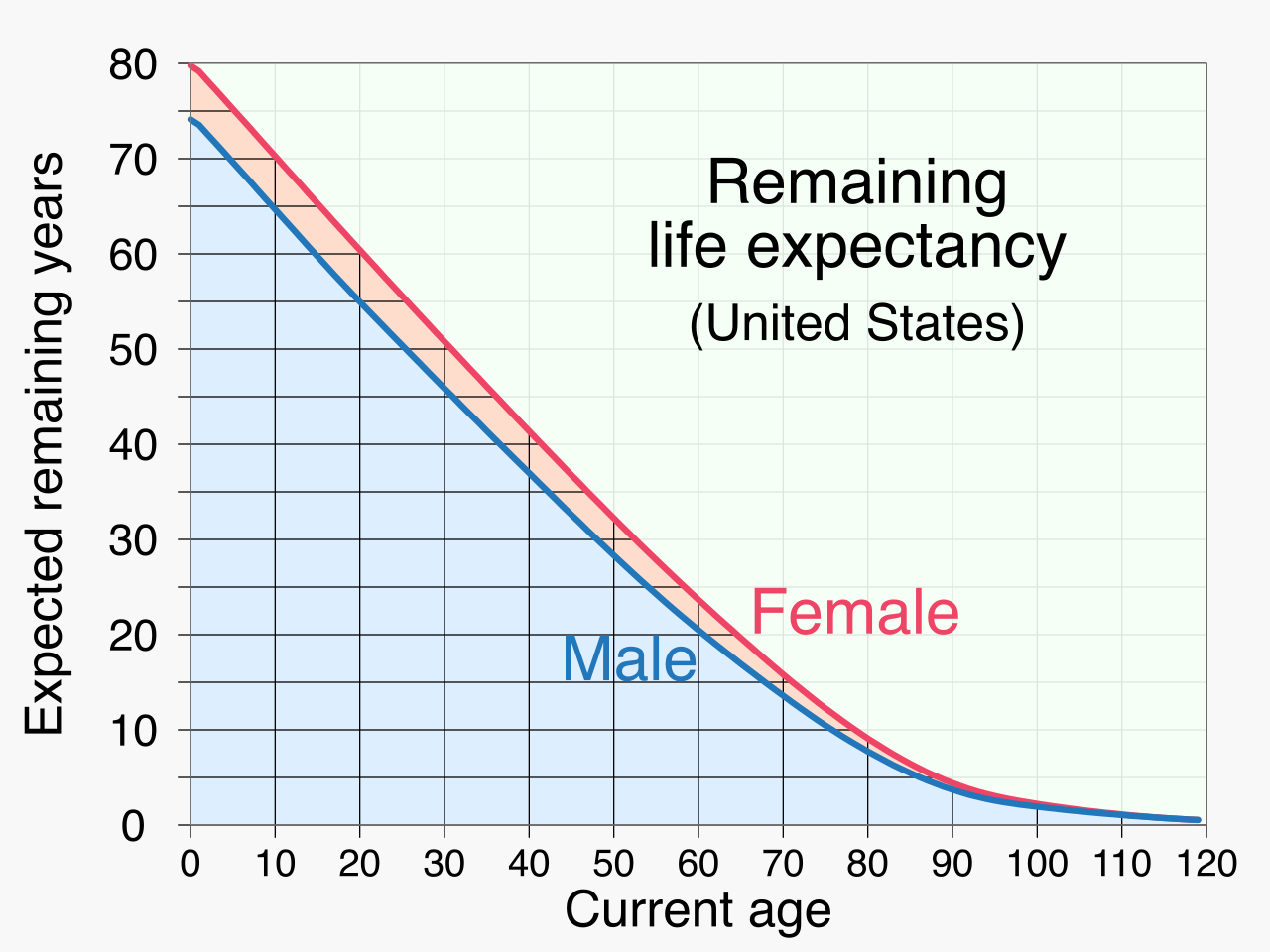
Bengen's research was later validated and expanded by the Trinity Study, which tested withdrawal rates over rolling 30-year retirement periods using historical market data. Both Bengen and the Trinity Study established critical baseline assumptions: the 4 percent rule assumes a mixed portfolio composition of equities and fixed income (typically 50/50 to 75/25), and it is strictly designed to sustain portfolio withdrawals over a 30-year period.
The Mathematics of Destruction: Sequence Risk
Why limit withdrawals to 4% when average historical market returns are 7% to 9%? Because in the real world, retirees do not experience "average" returns. They experience a specific sequence of returns.
Sequence of returns risk is the danger of experiencing negative portfolio returns early in retirement. When you are accumulating wealth, the order of returns does not matter due to the commutative property of multiplication. But once you begin taking distributions, the math breaks down. Negative returns early in retirement combined with steady withdrawals permanently reduce the principal available for future growth.
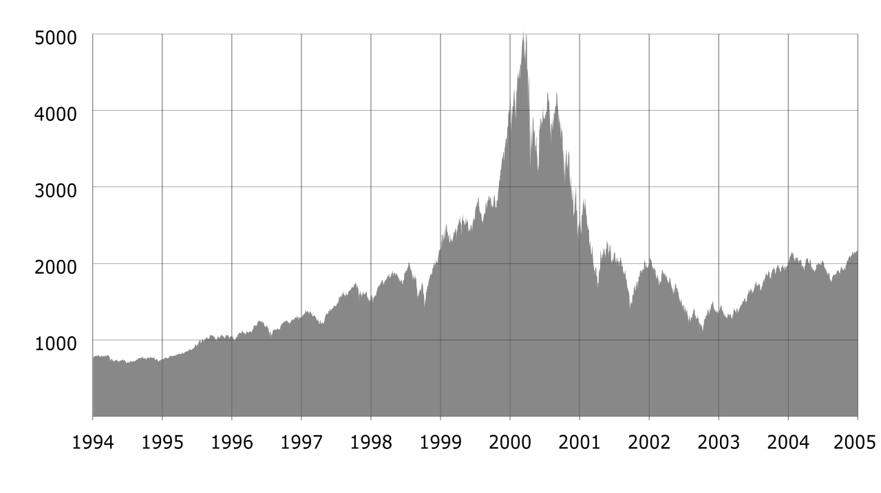
If a client retires and the market drops 20% in the first two years, they must sell a significantly larger number of shares to generate their $80,000 living expense. When the market eventually rebounds, the client has fewer shares left to capture the upside. The portfolio enters a death spiral. This is why the safe withdrawal rate is so low—it is a mathematical shock absorber designed to survive the worst historical sequences of returns, such as those beginning in 1929, 1966, or 2000.
Because blindly following the 4% rule through a major market crash requires superhuman psychological fortitude, elite financial planners use structural defenses to protect the portfolio from sequence risk.
1. Dynamic Withdrawal Strategies
Instead of adjusting withdrawals solely for inflation, dynamic withdrawal strategies adjust the annual distribution amount based on current portfolio performance.
A premier example is the Guyton-Klinger guardrail strategy, which applies decision rules to increase or decrease withdrawal rates based on initial withdrawal percentage thresholds.
- Capital Preservation Rule: If the market plummets and the withdrawal rate rises 20% above its initial target (e.g., an initial 4.0% rate becomes a 4.8% rate due to a shrinking portfolio balance), the retiree takes a pay cut, reducing their withdrawal by 10%.
- Prosperity Rule: If the market booms and the withdrawal rate falls 20% below the target, the retiree gets a 10% raise. This dynamic flexibility ensures the portfolio avoids the death spiral while allowing retirees to spend more during sustained bull markets.
2. The Bucket Strategy
To mitigate the behavioral panic that accompanies sequence risk, planners utilize a time segmentation or bucket strategy, which divides retirement assets into different pools based on the time horizon for needing the funds.
- Bucket 1 (Years 1-3): Short-term needs are funded with cash and cash equivalents to mitigate sequence of returns risk. If the market crashes the day after the client retires, their immediate living expenses are completely insulated. They are not forced to sell equities at a loss.
- Bucket 2 (Years 4-10): Intermediate needs are funded with fixed income and high-yield bonds, providing stable yield while allowing equities time to recover from standard market cycles.
- Bucket 3 (Years 11+): Long-term needs are funded with high-growth equities to outpace inflation. Because the client knows their next decade of spending is secured by Buckets 1 and 2, they can confidently let Bucket 3 weather severe market volatility.
3. The Flooring Strategy
For clients who cannot tolerate the risk of outliving their fundamental needs, planners utilize the flooring strategy, which matches guaranteed income sources like Social Security and annuities to cover a retiree's essential living expenses (housing, food, healthcare).
Once the "floor" of essential expenses is fully subsidized by guaranteed, lifetime income, the remainder of the portfolio can be invested more aggressively to fund discretionary expenses (travel, legacy). By securing the baseline, the flooring strategy completely neutralizes the catastrophic impact of sequence risk on a client's standard of living.
As a CFP professional, your mastery of these concepts is what separates a mere investment manager from a comprehensive financial architect. When you sit across from a client terrified by a plunging market, your ability to seamlessly execute a bucket strategy, maneuver around IRMAA tripwires using Roth reserves, and implement dynamic withdrawal guardrails is what transforms theoretical finance into their real-world financial security. You are not just managing their money; you are engineering their peace of mind.