Schedule Management and Critical Path
Not sure you’re ready?
Take the ~3-minute readiness diagnostic and see where you stand.
Every project is a race against the one resource you cannot requisition, borrow, or manufacture: time. Whether you are migrating a global enterprise to a new cloud infrastructure or constructing a commercial high-rise, Project Schedule Management includes the processes required to manage the timely completion of the project. To control a project, you must first map its anatomy. You cannot simply list thousands of tasks in a spreadsheet and hope they naturally align. Instead, we must mathematically model the flow of time, uncovering the invisible, critical arteries of work that dictate exactly when a project will finish and where its most dangerous bottlenecks lie.
Before we can analyze a schedule, we must build it. The foundational architecture of modern project scheduling relies on the Precedence Diagramming Method (PDM).
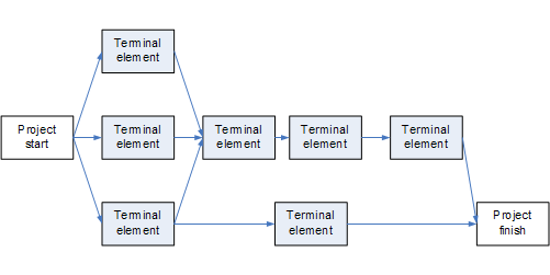
The Precedence Diagramming Method is a technique used for constructing a schedule model. It represents project activities as nodes (often drawn as boxes) and graphically links these activities by logical relationships to show the sequence of performance. You can think of it as a roadmap where the cities are the tasks, and the highways between them are the strict rules of sequence.
Logical Relationships: The Rules of Connection
In PDM, activities do not occur in a vacuum; they interact. We define exactly how one activity hands off to another through four specific logical relationships:
- Finish-to-Start (FS): A successor activity cannot start until a predecessor activity has finished.
- Example: You cannot begin testing a software module (successor) until the engineers have finished writing the code (predecessor). This is the most common relationship.
- Start-to-Start (SS): A successor activity cannot start until a predecessor activity has started.
- Example: You cannot start editing a documentary (successor) until you have at least started filming the footage (predecessor).
- Finish-to-Finish (FF): A successor activity cannot finish until a predecessor activity has finished.
- Example: The task of writing a user manual (successor) cannot completely finish until the development of the product itself (predecessor) has finished.
- Start-to-Finish (SF): A successor activity cannot finish until a predecessor activity has started.
- Example: A legacy database system cannot finish its shutdown process (successor) until the new replacement database has started operating (predecessor).
The Nature of Dependencies
Why do these logical relationships exist? As a project manager, you must understand whether a sequence is driven by the laws of physics, a signed contract, or merely a preference.
- Mandatory dependencies are logical relationships inherent in the nature of the project work, or they are contractually required. You physically cannot erect the walls of a building before pouring the foundation. It is non-negotiable.
- Discretionary dependencies are logical relationships established based on best practices or specific project team preferences. Your team might prefer to design the user interface before designing the backend database, even though they could theoretically be done in reverse.
- External dependencies involve a logical relationship between project activities and non-project activities outside the project team's control. Waiting for a city council to approve a building permit before you begin construction is an external dependency.
- Internal dependencies involve a logical relationship between project activities strictly within the control of the project team. If your internal QA team must test a machine before your internal marketing team photographs it, the team controls both tasks.
Fine-Tuning Time: Leads and Lags
Sometimes, a strict logical relationship needs a slight chronological adjustment.
- A lead is the amount of time whereby a successor activity can be advanced with respect to a predecessor activity. If a landscaping task has a 2-day lead on a building completion task, you are overlapping the work, starting the landscaping 2 days before the building is completely finished.
- A lag is the amount of time whereby a successor activity is delayed with respect to a predecessor activity. If you pour concrete, you must wait for it to cure before framing. That waiting period—where no active work is happening—is a lag.
Now we reach the mathematical heart of schedule management. The Critical Path Method (CPM) was originally developed in the late 1950s by Morgan R. Walker and James E. Kelley Jr. It is a schedule network analysis technique used to estimate the minimum project duration.
Imagine you are cooking a complex dinner. The salad takes 10 minutes, setting the table takes 5 minutes, but roasting the turkey takes 4 hours. No matter how fast you chop the lettuce or fold the napkins, dinner will not be ready for at least 4 hours. The turkey is your critical path.
By definition, the critical path is the sequence of activities representing the longest continuous path through a project network diagram. Because it is the longest path of sequential work, the critical path determines the shortest possible time required to complete the entire project.
The Forward and Backward Pass
To analyze the network, CPM uses an algorithm requiring two sweeps through your project data:
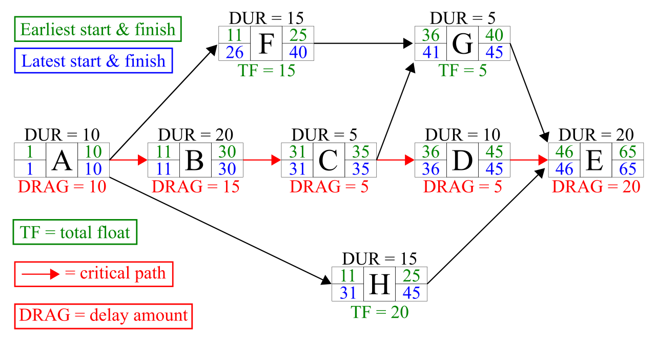
- The Forward Pass: We sweep forward from the start of the project to the end. A forward pass calculates the Early Start (ES) and Early Finish (EF) dates for all project activities.
- The Early Start date is the earliest possible point in time an activity can begin based on schedule network logic.
- The Early Finish date is the earliest possible point in time an activity can finish based on schedule network logic.
- The Backward Pass: We sweep backward from the project's end date to the beginning. A backward pass calculates the Late Start (LS) and Late Finish (LF) dates for all project activities.
- The Late Start date is the latest possible point in time an activity can start without delaying the project finish date.
- The Late Finish date is the latest possible point in time an activity can finish without delaying the project finish date.
Understanding Float (Slack)
When you compare the early dates and late dates, you discover flexibility—a concept called float.
Total Float is the amount of time an activity can be delayed without delaying the overall project finish date.
Formulas for Total Float:
- Late Start minus Early Start (LS−ES)
- Late Finish minus Early Finish (LF−EF)
If a task can start as early as Day 10, but doesn't strictly need to start until Day 15 without pushing the project end date, it has 5 days of total float.
Crucially, activities on the critical path typically have zero total float. They have no flexibility. A one-day delay on the critical path equals a one-day delay for the entire project finish date.
Do not confuse Total Float with Free Float. Free float is a highly localized metric: it is the amount of time an activity can be delayed without delaying the Early Start date of any immediate successor activity.
Schedule Risk and Multiple Paths
Network diagrams are rarely perfectly linear. What happens if a project schedule network diagram has multiple critical paths running concurrently?
The existence of multiple critical paths increases the overall schedule risk of a project. If you have three separate critical paths, you have three separate sequences of work that can instantly delay your project if anything goes wrong.
Furthermore, you must watch the near-critical path, which is a sequence of activities with a very small amount of total float. A near-critical path will become the new critical path if its activities experience delays exceeding their total float. A good project manager treats near-critical paths with the same deep respect as the critical path itself.
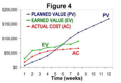
Building the CPM network is a planning exercise. But what happens when the project starts, the world intervenes, and execution gets messy? We must measure reality against our theoretical baseline. For this, we use Earned Value Management (EVM) metrics.
To calculate schedule performance, EVM compares two fundamental financial metrics linked to time:
- Planned Value (PV): This represents the authorized budget assigned to the scheduled work expected to be accomplished. It is where you should be according to your calendar.
- Earned Value (EV): This represents the authorized budget assigned to the scheduled work that has actually been completed. It is the physical reality of what you have built.
Schedule Variance (SV)
Schedule Variance is an Earned Value Management metric used to measure overall schedule performance. It asks a simple question: In terms of value, how far off the schedule are we?
Formula: Schedule Variance (SV)=Earned Value (EV)−Planned Value (PV)
| If Schedule Variance is... | It means... |
|---|---|
| Positive (> 0) | The project is currently ahead of schedule. You have earned more value than you planned to at this point in time. |
| Exactly Zero (= 0) | The project is perfectly on schedule. |
| Negative (< 0) | The project is currently behind schedule. You have accomplished less than planned. |
Schedule Performance Index (SPI)
While Variance gives you a raw number, the Schedule Performance Index (SPI) is an Earned Value Management metric used to measure schedule efficiency. It tells you at what rate you are accomplishing the work.
Formula: Schedule Performance Index (SPI)=Earned Value (EV)÷Planned Value (PV)
| If Schedule Performance Index is... | It means... |
|---|---|
| Greater than 1.0 | More work was completed than originally planned. You are operating highly efficiently. |
| Exactly equal to 1.0 | The project work is proceeding exactly as planned. |
| Less than 1.0 | Less work was completed than originally planned. You are operating inefficiently and falling behind. |
Imagine you check your metrics. Your SPI is 0.85 and your Schedule Variance is heavily negative. The project is behind schedule, but the final deadline is immovable. What do you do?
You must compress the schedule. Schedule compression techniques shorten the project schedule duration without reducing the project scope. We do not get to do less work; we just have to do it faster. We achieve this through two primary methods applied directly to activities on the critical path:
1. Crashing
Crashing is a schedule compression technique used to shorten the schedule duration by adding extra resources.
- The Reality: If you have two painters painting a room, crashing means hiring two more painters so the room is finished in half the time. You are throwing money at the problem. Therefore, the crashing schedule compression technique typically results in increased overall project costs.
2. Fast Tracking
Fast tracking is a schedule compression technique where activities normally done in sequence are instead performed in parallel.
- The Reality: Instead of waiting for the software backend to be 100% finished before starting the frontend design, you start the frontend design while the backend is still being built. You are changing a Finish-to-Start relationship to a Start-to-Start relationship with a lead.
- The Risk: Because you are performing dependent tasks simultaneously, the fast tracking schedule compression technique often results in increased project risk. If the backend engineers realize they need to change the database architecture, the frontend designers will have to throw away their parallel work and start over. Thus, fast tracking frequently results in increased project rework.
Final Synthesis
Mastering Project Schedule Management means understanding time as a tangible, mathematical structure. By mapping logical dependencies (PDM), finding the longest sequential path of work (CPM), aggressively monitoring progress through EVM metrics (SV and SPI), and knowing precisely how to squeeze time when deadlines loom (Crashing and Fast Tracking), you transform from a passive observer of a calendar into an active architect of project delivery.