Coordinate Geometry
Not sure you’re ready?
Take the ~3-minute readiness diagnostic and see where you stand.
Coordinate geometry is the Rosetta Stone of secondary mathematics. It is the precise arena where the rigid, logical axioms of classical geometry translate perfectly into the fluid, operational machinery of algebra. For the aspiring mathematics educator, mastering the coordinate plane is not merely an exercise in memorizing formulas; it is about learning to reveal to students the profound truth that every shape has an equation, and every equation has a shape. When a student struggles to visualize an abstract algebraic concept, the Cartesian plane provides the visual proof. Your command of this translation dictates how well your future students will bridge the gap between calculating a result and genuinely understanding the space it occupies.
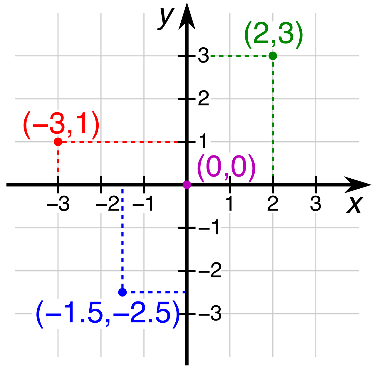
To operate in the coordinate plane, we must first establish how we measure the space between two points. Students frequently view the distance formula as a chaotic jumble of subscripts, squares, and square roots to be memorized by rote. Your job is to pull off the mask and show them what it really is: an old friend.
The distance formula in the coordinate plane is a direct application of the Pythagorean theorem. When we want to find the distance between two points (x1,y1) and (x2,y2), we are simply drawing a right triangle whose hypotenuse connects those two points. The horizontal leg of this triangle has a length of ∣x2−x1∣, and the vertical leg has a length of ∣y2−y1∣.
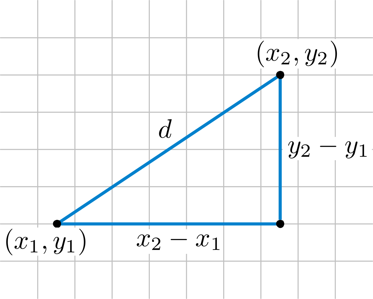
The Distance Formula The distance d between two points (x1,y1) and (x2,y2) in the coordinate plane is calculated using the formula: d=(x2−x1)2+(y2−y1)2
Because we square the differences, the order of subtraction does not matter, and the result is always a non-negative distance—exactly what we expect when applying a2+b2=c2.
The Midpoint as an Average
Once we know how far apart two points are, the next logical question is how to find the exact center of that distance. Often, textbooks present the midpoint formula as another distinct geometric theorem. However, a much more powerful, intuitive framing for your students is rooted in basic statistics.
The Midpoint Formula The midpoint of a line segment with endpoints (x1,y1) and (x2,y2) is the point: (2x1+x2,2y1+y2)
Why does this work? Because the x-coordinate of a line segment's midpoint is simply the arithmetic mean of the x-coordinates of the segment's endpoints. Similarly, the y-coordinate of a line segment's midpoint is the arithmetic mean of the y-coordinates of the segment's endpoints. If one endpoint is at an x-coordinate of 2 and the other is at 10, the "middle" is exactly the average: 6. Framing the midpoint as an average demystifies the coordinate plane, grounding geometric concepts in basic arithmetic intuition.
Finding a midpoint is simply partitioning a segment into a 1:1 ratio. But what if we want to divide a segment into unequal parts? What if a problem asks for a point that is exactly two-thirds of the way along a line? This introduces the concept of the directed line segment.
A directed line segment has a specific starting endpoint and a specific ending endpoint. In undirected geometry, segment AB and segment BA are identical entities. On the coordinate plane, however, the order of endpoints in a directed line segment defines the direction of the segment. Moving from A to B is a completely different journey than moving from B to A.
Partitioning a directed line segment from point A to point B in a ratio of a:b means finding a point P such that the ratio of the length of AP to the length of PB is ba.
The Intuitive "Fractional Distance" Approach
The most common cognitive trap students fall into is confusing the ratio with the fraction of the total journey. If we partition a segment in a 2:3 ratio, the point P is not 32 of the way down the line.
Instead, a point partitioning a directed line segment into a ratio of a:b divides the total length of the segment into a+b equal parts. Therefore, the fractional distance from the starting point to the partition point in a segment divided into a ratio of a:b is equal to a+ba. In our 2:3 example, the total journey is 2+3=5 parts, making the fractional distance 52 of the way from A to B.
Once the fractional distance is understood, the coordinates of the partition point can be found by adding that fraction of the total horizontal and vertical changes to the starting coordinates:
The Fractional Distance Partition Formulas To find the x-coordinate of a point partitioning a directed segment from (x1,y1) to (x2,y2) in a ratio of a:b, use the formula: x=x1+(a+ba)(x2−x1)
To find the y-coordinate of a point partitioning a directed segment from (x1,y1) to (x2,y2) in a ratio of a:b, use the formula: y=y1+(a+ba)(y2−y1)
This translates plainly to: Start at the beginning (x1), then add your fractional progress (a+ba) of the total distance traveled (x2−x1).
The Algebraic "Section Formula" Approach
While the fractional distance approach builds excellent conceptual understanding, there is a more streamlined algebraic approach, often referred to as the Section Formula.
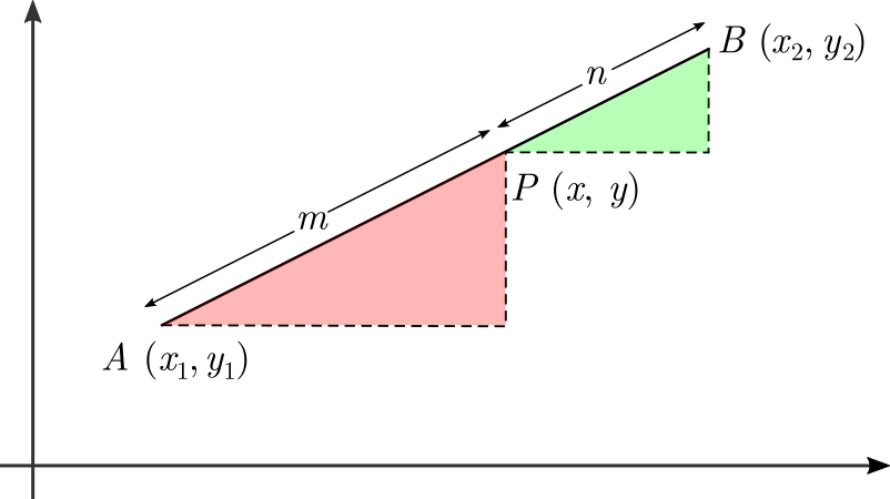
Alternative Section Formulas (Ratio m:n) An alternative section formula for the x-coordinate of a point partitioning a segment from (x1,y1) to (x2,y2) in ratio m:n is: x=m+nm⋅x2+n⋅x1
An alternative section formula for the y-coordinate of a point partitioning a segment from (x1,y1) to (x2,y2) in ratio m:n is: y=m+nm⋅y2+n⋅y1
Notice how this formula takes the form of a weighted average, "crossing" the ratio values with the opposite coordinates. As a teacher, it is powerful to present both methods:
| Approach | Pedagogical Advantage | Mental Model |
|---|---|---|
| Fractional Distance | Builds geometric intuition and mirrors real-world travel (e.g., "driving 2/5 of the way to a destination"). | Position=Start+(Fraction×Change) |
| Section Formula | Highly efficient for algebraic manipulation; prevents calculation errors with negative coordinates. | Position=Weighted Average of Endpoints |
As we move from lines to curves, coordinate geometry continues to rely entirely on the foundations we just built. Take the circle. In classical geometry, a circle is defined as the set of all points in a plane that are equidistant from a given center point.
In the coordinate plane, the standard equation of a circle expresses this precise geometric definition: every point (x,y) on the circle is exactly a distance of r from the center point (h,k).
Because a circle is fundamentally just a statement about distance, the standard equation of a circle is derived directly from the distance formula. If we take our distance formula, d=(x2−x1)2+(y2−y1)2, replace our two points with a fixed center (h,k) and an arbitrary point (x,y), and replace the distance d with the radius r, we get r=(x−h)2+(y−k)2. Squaring both sides removes the radical, yielding one of the most elegant equations in mathematics.
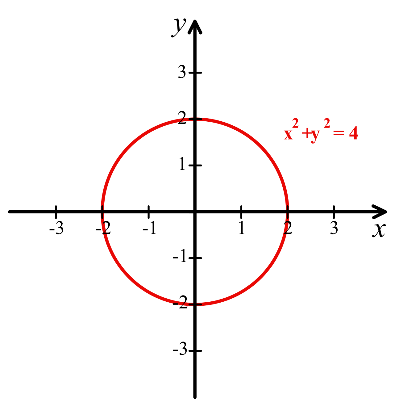
Standard Equation of a Circle The standard equation of a circle in the coordinate plane is: (x−h)2+(y−k)2=r2
In this standard equation:
- The point (h,k) represents the center of the circle.
- The variable r represents the radius of the circle.
Unpacking the General Equation
While the standard equation is beautiful and geometrically informative, test designers and real-world algebraic systems rarely hand us equations in this neat package. Often, the equation is expanded and rearranged into what is known as the general equation.
The general equation of a circle is written in the expanded form: x2+y2+Dx+Ey+F=0
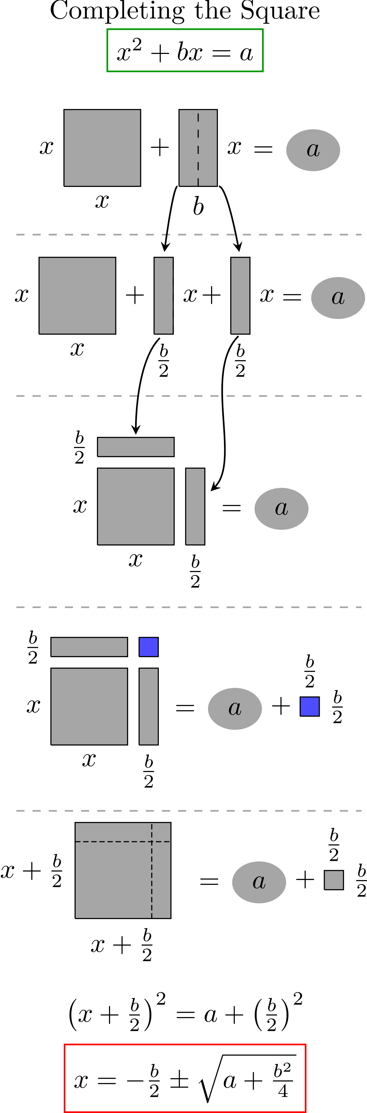
Looking at this form, the geometric features of the circle (the center and the radius) are entirely hidden. To extract the spatial meaning from this algebraic string, we must reverse the expansion. The algebraic process of completing the square is used to convert the general equation of a circle into the standard equation of a circle. By grouping the x-terms and y-terms and completing the perfect square trinomials for each, you reconstruct the (x−h)2 and (y−k)2 groupings, shifting the remaining constants to the right side of the equals sign to reveal r2.
Interpreting Degenerate Cases
As you guide students through completing the square, you will inevitably encounter cases where the algebra yields a surprising result on the right side of the equals sign. The value of r2 is the ultimate arbiter of what the equation actually represents in the physical coordinate plane.
- The Standard Circle (r2>0): This generates our expected, visible circle with a quantifiable radius r=r2.
- The Point Circle (r2=0): If the radius squared value (r2) in a circle's standard equation is zero, the graph represents a single point instead of a circle. Geometrically, a circle with a radius of zero has collapsed onto its center (h,k).
- The Imaginary Circle (r2<0): If the radius squared value (r2) in a circle's standard equation is a negative number, the equation has no real solutions and does not graph a visible circle. Since the sum of two squared real numbers (x−h)2+(y−k)2 cannot be negative, there are no points in the real Cartesian plane that satisfy this condition.
In your classroom, treating these edge cases not as "trick questions" but as logical boundaries of the mathematics will foster deeper algebraic reasoning. You are teaching students that the coordinate plane is not just a drawing board—it is a strict, logical interpreter of algebraic truth.